|
|
|
|
|
| Finds optimum operating point when the number of variables is large and there are a variety of interactions between them |
To illustrate the concepts in a very simple example, assume that we're running a furniture factory. This model has a profit equation with 2 terms, and has 2 constraint equations, requiring a profit computation at 3 places. By comparison, a plywood mill has a profit equation with 3400 terms, about 4600 constraint equations, and 12,000 places to compute a profit!
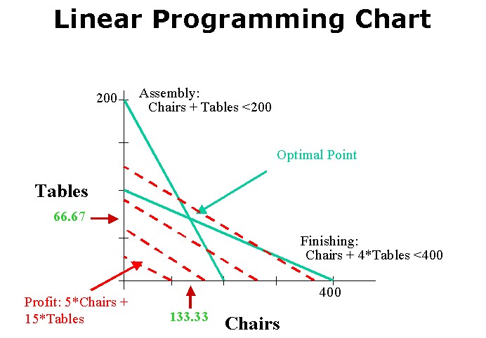
Our Assembly area can put together 200 chairs and/or tables a day; our finishing area can do 100 Tables or 400 Chairs a day. These become our constraints, shown in blue above -- we can't have an operating point to the upper right of these lines.
Our gross margins on chairs is $5, on tables $15. The gross margin equation is shown in dotted red for a few sample operating points.
The optimal point is at that place where the profit is maximized, but within the constraint boundary. The solver engine moves the profit line in small increments until it hits constraints.
Notice that the optimum point requires making fractional chairs and tables -- clearly not possible. But the optimum operating point is +- 1 chair/table away from this point and is easily analyzed as a second step.
In the real world, there are hundreds of dimensions to the chart, and hundreds of constraint equations, and we can no longer visualize the optimum operating point. That's why we use Linear Programming technology, included with Enterprise Optimizer.
If we are required to keep the ratio of tables and chairs within certain bounds, that produces a different constraint (example).
|
Send mail to
webmaster@bytedesign.com with
questions or comments about this web site.
|